Differential Drive – Home-Grown Robotics

There are many different robotics drivetrains, one of the most common drive types that you will encounter is the Differential Drive. This control scheme is praised for its simplicity, ease of implementation, and ability to be used in many situations. This system is simply defined by two wheels independently controlled by their own motor.

Some examples of differential drive robots include, but are not limited to:

Project LiftOff
Edison
iRobot Roomba
e-puck
Amazon Warehousing Robots (Kiva Systems)

In this article I want to bring a more nuanced understanding of this style of robot, discuss the kinematic model show how it is represented as a mathematical model, and pair this information with my robot kit to show how we can improve its performance with simple control systems. Let’s begin!

The Kinematic Model

Let’s establish our known constraints for a simple robot

Right away we know it has a pair of wheels that share an axis, these wheels are allowed to spin independently of each other either in the positive or negative direction of our choice. Each wheel will have the same radius, $r$ , and the distance between the wheels will be defined as, $l$ .

D is the distance traveled (in the same units as d). $D * RPM$ is your speed in $Revolutions/Minute$ . Convert this as needed for your application. If we assume perfectly matched wheels and velocity we could use the above formula to determine distance traveled. Of course, life is not so easy on us due to the differences in terrain, wheel size, traction, encoder accuracy, etc.

Intuitively, we understand that if both wheels spin with the exact same angular velocity, our system will move forward perfectly straight, and if perfectly opposed (negative and positive with the same magnitude) it will turn in place. Therefore, if we were to cause a difference between the angular velocity’s of the wheels $V_L$ or $V_R$ , we would get a corresponding change in the angular velocity of the system, $\omega$ , hence we will see our robot make a curved path. Now, you can visualize this just like when you draw a circle or arc with a compass, the marking end is the robots’ path and the anchor is where the center of the curve is. This anchor point is known as the Instantaneous Center of Curvature (I.C.C). This isn’t going to be useful to us if we can’t control this behavior or predict where our robot is going to go, we need some equations and feedback to assist us.

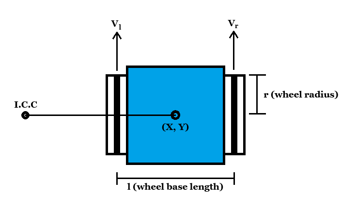
Kinematic Model

$\omega(R + \frac{l}{2}) = V_r$

$\omega(R - \frac{l}{2}) = V_l$

$\omega$ remains constant for both wheels along the I.C.C. l is the distance between the wheel centers, R is the signed distance from the I.C.C to the midpoint of the chassis, and V_r, V_l are the right and left wheel speeds respectfully.

You can reorder the equations to solve for R and $\omega$ at any point in time:

$R =\frac{l}{2} \frac{V_l + V_r}{V_r - V_l}$

$\omega = \frac{V_r - V_l}{l}$

With these equations, we can see our intuitions about the motion of the system be shown:

If $V_r = V_l$ , then the robot will travel in a straight path. $R$ will become infinitely large, and angular velocity must go to 0.
If $V_r = -V_l$ , $R$ goes to 0, and the robot is turning in place depending on which direction the wheels are turning opposite of each other.
If $V_r = 0$ , or $V_l = 0$ , the robot will rotate about the wheel that is not moving (left or right), and $R$ becomes $l/2$ .

Forward Kinematics

Kinematics overall describes the robot’s motion. Forward kinematics is used to calculate the position and orientation of the robot when given a kinematic chain with multiple degrees of freedom. (https://opentextbooks.clemson.edu/wangrobotics/chapter/forward-kinematics/).

The object is rigid, such that its constituent points maintain a constant relative position with respect
to each other and to the object’s coordinate frame This holds under any translation and rotation
applied to the rigid body Point abstraction can be applied (note: does not
apply to soft or humanoid robots)

A robot of any single-body shape can be “reduced” to a point, selected as reference point

The configuration of a non-omnidirectional mobile robot in a two-dimensional coordinate systems is fully defined by its position (x, y) where the Orientation angle is $\theta$ and the triple $q=(x, y, \theta$ ) is the robot pose.